NeuraIPS2022, facebookresearch에서 Theseus 라는 이름으로 differentiable non-linear optimization library를 공개했다.
프로젝트 페이지의 링크는 다음과 같다. https://sites.google.com/view/theseus-ai/
Theseus
Theseus is an efficient application-agnostic library for building custom nonlinear optimization layers in PyTorch to support constructing various problems in robotics and vision as end-to-end differentiable architectures. See summary thread on 🐦 Twitter
sites.google.com
주 목적은 딥러닝 네트워크를 학습 시에 명확히 있는 GT를 이용해서 학습하는 것이 아니라, 최적화를 통해 얻어낸 값을 GT로 사용하여 학습할 수 있도록 하는 것 같다.
즉, 딥러닝 학습 과정에 최적화 알고리즘이 끼어들 수 있도록 non-linear optimization library를 differentiable한 형태로 정리하고 이를 pytorch와 쉽게 호환/연동되도록 했다.
형태를 보면, 최적화 알고리즘을 구현하는 것 외에 이를 TheseusLayer라는 이름으로 wrapping하는 과정이 포함되어 있다.
눈에 띄는 것은 최적화 알고리즘을 구현하는 파트를 python으로 구현할 수 있도록 해두었고, pytorch와 간단히 호환되면서 기존의 유명한 library, CERES 대비 속도가 빠르다고 주장하는 것이다.
최적화 알고리즘을 구현하려고 하면, 보통 c++로 제공되는 library가 많아 c++에 익숙치 않다면 애를 먹는 경우가 많다. (ceres가 그렇다. 설치도 까다롭고...입문도 그렇고...)
pytorch를 이용해서 구현을 할 수 있긴 하지만 optmizer가 딥러닝용으로 사용되던 optimizer 뿐이고 gauss-newton이나 lavenberg-marquardt optimizer를 기대할 경우에는 구현이 어렵다.
게다가 SO3나 SE3 값이 최적화 대상일 경우, parameterization하는 건 별도의 이슈로 남아있다.
그런 측면에서, Theseus를 이용하면 최적화 알고리즘을 간단히 구현할 수 있을 것이라 기대된다.
대표적으로 최적화를 많이 사용하는 부분이 3D vision에서 카메라의 자세를 추정하는 부분인데, 이 글에서는 Theseus를 이용해 간단히 pose estimation 코드를 작성해보면서 문법과 성능/속도를 맛보기 해보고자 한다.
0. 예제 설명
카메라 자세 추정에서 가장 가벼운 세팅은 3D point와 이에 대응되는 2D point, N 쌍을 알고 있을 때이다.
opencv solvePnP로 간단히 계산할 수 있는 세팅과 같은데, 이를 Theseus optimizer로 만들어 풀어보고자 한다.
간단히 PnP 문제는 SVD를 이용해 풀 수 있는 least-square 문제로 아는데 이와 값, 속도를 비교해보는 예제이다.
1. 준비물
80개의 점이 있는 visual marker를 캘리브레이션된 카메라로 촬영했다. marker 상에 있는 3D point의 좌표와 이미지 상에서 검출된 marker point의 2D 좌표를 저장한 파일이다.
2. 데이터 준비
사용된 이미지는 굳이 필요하지 않아서 포함되어 있지 않고, 사용할 intrinsic calibration 값은 코드에 기록해두었다. 편의 상 zero distortion을 가정했다.
material_dir = "PATH_TO_DATA_DIR"

'''
step0 : data preparation

short description
check dtype of variables. unify all dtypes as np.float32 or np.float64.
'''
pt3ds_np = np.load(os.path.join(material_dir, "tag3ds.npy")).astype(np.float32) # [80, 3]
pt2ds_np = np.load(os.path.join(material_dir, "tag2ds.npy")).astype(np.float32) # [80, 2]

img_w, img_h = 6720, 4480
num_points = np.shape(pt3ds_np)[0]

fx, fy, cx, cy = 9940.201263283288, 9941.26059620391, 3326.074229221311, 2203.6479161585257
K_np = np.array([[fx, 0, cx],
                 [0, fy, cy],
                 [0, 0, 1]], dtype=np.float32)
dist_np = np.array([0.0, 0.0, 0.0, 0.0, 0.0], dtype=np.float32) # let assume zero distortion for simplicity

pt3ds_torch = torch.from_numpy(pt3ds_np) # [80, 3]
pt2ds_torch = torch.from_numpy(pt2ds_np) # [80, 2]
K_torch = torch.from_numpy(K_np) # [3, 3]
dist_torch = torch.from_numpy(dist_np) # [5,]
3. Variable 준비
아래 주석 참고. initialization 값은 아무렇게나 사용해도 되지만, 현 세팅에서 카메라 translation을 (0, 0, 0)으로 할 경우 뒤 과정에서 zero dividing이 생기기 때문에 임의로 z값만 40cm로 설정함.
'''
step1 : variable preparation

There are two types of Variables
(1) optim_vars : target variables of optimization which are updated - transformation 4x4 matrix in this case
(2) aux_vars :  supporting variables of optimization which are not updated. - 3d points, 2d points and intrinsic parameters in this case

short description
th.SO3: variable for SO3. similar concept to quaternion parameterization of CERES
th.SE3 : variable for SE3. SO3 + translation XYZ
th.Variable : general variable

theseus uses (qw, qx, qy, qz) convention for SO3 and (tx, ty, tz, qw, qx, qy, qz) convetion for SE3
th.SO3, th.SE3 can be initialized by both quaternion form and matrix form. refer below codes.
'''

### all theseus variables should have batch dimension
T_cw = th.SE3(x_y_z_quaternion=torch.FloatTensor([[0.0, 0.0, 0.40, 1.0, 0.0, 0.0, 0.0]]), name="T_cw")
# T_cw = th.SE3(tensor=TRANSFORMATION4X4_MATRIX, name="T_cw") # tensor [1, 4, 4]
pt3ds = th.Variable(pt3ds_torch.unsqueeze(dim=0), name="obj_points") # [1, 80, 3]
pt2ds = th.Variable(pt2ds_torch.unsqueeze(dim=0), name="img_points") # [1, 80, 2]
K = th.Variable(K_torch.unsqueeze(dim=0), name="K_th") # [1, 3, 3]

### grouping in list
optim_vars = [T_cw]
aux_vars = [pt3ds, pt2ds, K]
4. cost function 준비
원하는 형태의 cost를 계산하는 함수를 torch로 구현하면 된다. 대신 입력은 theseus variable로부터 들어와야 하는데, 이는 간단히 .tensor를 호출해서 얻은 torch tensor를 사용하면 된다.
'''
step2 : cost function preparation

short description
build error_fn (loss_fn) based on torch. easy.
replace the input of error_fn as th_varaible.tensor
'''
def project_points(pt3ds, T34, K):
    pt3ds_h = torch.cat([pt3ds, torch.ones_like(pt3ds[:,:, :1])], dim=2)
    cam_points = torch.matmul(T34, pt3ds_h.permute(0, 2, 1))
    img_points = torch.matmul(K[:, :3, :3], cam_points).permute(0, 2, 1)
    img_points = img_points / img_points[:, :, 2:] # be careful. zero dividing.
    return img_points[:, :, :2]

def error_fn(optim_vars, aux_vars):
    T_cw = optim_vars[0]
    obj_points = aux_vars[0]
    img_points = aux_vars[1]
    K = aux_vars[2]
    proj_img_points = project_points(obj_points.tensor, T_cw.tensor, K.tensor) # access tensors inside theseus variables using .tensor.
    error = proj_img_points - img_points.tensor
    error = torch.sqrt(torch.sum(error**2, dim=2)) # do not average values. maintain second dimension. [1, 80]
    return error

# similar to CERES AutoDiffCostFunction.
cost_function = th.AutoDiffCostFunction(optim_vars, error_fn, num_points, aux_vars=aux_vars, name="cost_fn")
5. objective 준비
'''
step3 : objective preparation

short description
wrapping cost_fn with th.Objective
if there are multi cost_fn for optimization, you can add more cost_fn and weight them with cost_weight
'''
objective = th.Objective()
objective.add(cost_function)
optimizer = th.GaussNewton(
    objective,
    max_iterations=100,
    step_size=0.5,
)
6. TheseusLayer 준비
'''
step4 : TheseusLayer preparation

short description
wrapping Objective weith th.TheseusLayer()
it become layer form of torch such as nn.Linear()
'''
th_optim = th.TheseusLayer(optimizer)
7. 실행 및 평가
'''
step5 : running
'''
th_start = time.time()
with torch.no_grad():
    updated_inputs, info = th_optim.forward()
th_end = time.time()
T_cw_th = updated_inputs["T_cw"][0].numpy()

'''
evaluation
'''
### opencv solvePnP result
cv_start = time.time()
ret, rvec, tvec = cv2.solvePnP(pt3ds_np, pt2ds_np, K_np, dist_np)  # kg
cv_end = time.time()

R_cw, _ = cv2.Rodrigues(rvec)
t_cw = tvec.reshape(-1)
T_cw_cv = np.eye(4)
T_cw_cv[:3, :3] = R_cw
T_cw_cv[:3, -1] = t_cw

def eval_reproj_erorr(T_cw, K, dist, obj_points, img_points):
    rvec = Rot.from_matrix(T_cw[:3, :3]).as_rotvec()
    tvec = T_cw[:3, -1]
    proj_img_points, _ = cv2.projectPoints(obj_points, rvec, tvec, K, dist)
    proj_img_points = proj_img_points[:, 0, :]
    error = np.linalg.norm(img_points - proj_img_points, axis=1)
    error = np.mean(error)
    return error

error_cv = eval_reproj_erorr(T_cw_cv, K_np, dist_np, pt3ds_np, pt2ds_np)
error_th = eval_reproj_erorr(T_cw_th, K_np, dist_np, pt3ds_np, pt2ds_np)

print("Evaluation result")
print(f"OPENCV solvePnP reprojection error : {error_cv} in {cv_end - cv_start} secs")
print(f"Theseus optimization reprojection error : {error_th} in {th_end - th_start} secs")
8. 결과

결과를 보면 0.16초에 CPU를 통한 최적화가 완료되었다. 체감 상 느린 편은 아닌 것 같다. 결과 값도 괜찮고.
OPENCV는 문제 특성 상 SVD로 단순 계산이 가능하기 때문에 속도가 보다 빠른 것이지 않을까 싶은데 뭐 나쁘지 않은 것 같다.
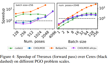
논문에서 언급한 바로, 병렬 연산이 지원돼서 속도 측면에서 빠르다는 것이지 현재처럼 batch 1일 경우에는 ceres 대비 속도가 느린 건 맞다.
9. 결론
결론적으로 Theseus를 자주 사용하게 될 것 같다. 최적화를 구현할 일이 생각보다 빈번한데 이 때마다 ceres 어떻게 쓰지... 고민할 것 없이 빠르게 Theseus로 구현하면 좋을 것 같다.
10. Note
위 예제코드는 CPU에서 동작하도록 되어있다. GPU를 사용하고 싶을 경우, "3. Variable 준비" 에서 cuda tensor를 이용해 variable을 생성하고 "5. objective 준비" 에서 생성된 objective를 .to(device="cuda:0")을 통해 cuda device로 옮겨준 뒤 실행하면 된다.
'Knowhow > Vision' 카테고리의 다른 글
| Tensorboard를 이용한 pb 파일 시각화 (0) | 2023.02.03 |
|---|---|
| Basalt 사용, tag 규격 정하기, 이미지로부터 rosbag 파일 만들기 (0) | 2023.01.19 |
| COLMAP[CLI] SfM/MVS with known camera parameters and poses (0) | 2022.07.14 |
| COLMAP write txt files in python (0) | 2022.07.13 |
| COLMAP read bin/txt/ db files in python (0) | 2022.07.13 |