Neural Implicit Surface Evolution 논문에서 level set equation을 이용해 두 형상 간의 interpolation을 implicit function으로 표현했을 경우 얻을 수 있는 이득에 적잖이 놀랐다.
문득, level set equation에서 a(t)로 표현되는 어떤 한 point의 시간에 따른 trajectory가 들어있는 것을 보고,
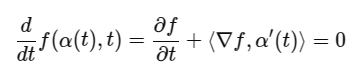
학습이 완료된 상태라면 저 a'(t) (a(t)는 계산 못함) 를 역계산할 수 있을텐데, 그러면 한 위치 x에서 a'(t)를 따라 적분해나간다면 x의 trajectory를 표현할 수 있는거 아닌가? 라는 궁금증이 생겼다.
만약 그게 된다면, geometry A 의 vertex들을 입력으로 넣고 a'(t)를 이용해 trajectory를 따라 이동시켜서 geometry B에 도착한 결과물을 얻을 수 있는 것인데 그게 바로 A-to-B correspondence가 되는게 아닌가? 라는 생각까지 이르렀다.
그래서 직접 해봤다.
a'(t) 계산하기

본래 LSE를 뒤집기만 하면 a'(t)는 구할 수 있기 때문에 쉽다. 그리고 우변의 값들은 이미 gradient가 흐른 상황이라면 가볍게 꺼내서 얻을 수 있는 값이니 계산까지도 어렵지 않음
def flow_field(f_model, x, t):
    x = x.clone().detach().requires_grad_(True)
    t = t.clone().detach().requires_grad_(True)
    t_expand = t.view(-1, 1).expand(-1, 1)

    input_xt = torch.cat([x, t_expand], dim=-1)  # (N, 4)

    f_val = f_model(input_xt, skip_detach=True)["model_out"]  # (N, 1)
    ones = torch.ones_like(f_val)

    # Spatial gradient ∇f
    grad_x = torch.autograd.grad(f_val, x, grad_outputs=ones, create_graph=True, retain_graph=True)[0]  # (N, 3)

    # Temporal gradient ∂f/∂t
    grad_t = torch.autograd.grad(f_val, t, grad_outputs=ones, create_graph=True)[0].view(-1, 1)  # (N, 1)

    norm_sq = (grad_x ** 2).sum(dim=1, keepdim=True) + 1e-6
    velocity = - grad_t * grad_x / norm_sq  # (N, 3)

    return velocity
나는 이렇게 계산하는 코드를 짰다. 코드는 NISE에다가 갖다 붙여서 썼고.
적분해서 trajectory 만들기
    start_verts, start_faces, _, _ = create_mesh(
                        model,
                        t=training_data_config["timesampler"]["range"][0],
                        N=256,
                        device=device
                    )

    indices = np.random.choice(start_verts.shape[0], size=8000, replace=False)
    start_verts = start_verts[indices]  # shape: (8000, 3)
    start_verts = torch.from_numpy(start_verts.astype(np.float32)).cuda()

    num_steps = 1000
    x = start_verts.clone().detach()
    t = torch.full((x.shape[0],), training_data_config["timesampler"]["range"][0], dtype=torch.float32, device=x.device)
    dt = (training_data_config["timesampler"]["range"][1] - training_data_config["timesampler"]["range"][0]) / num_steps
    trajectory = [x.clone().detach().cpu().numpy()]

    model.eval()
    for step in range(num_steps):
        x = x.clone().detach().requires_grad_(True)
        v = flow_field(model, x, t)
        x = x+dt*v
        t = t+dt
        trajectory.append(x.clone().detach().cpu().numpy())
flow_field 함수에서 뱉어주는 a'(t)를 아주 작은 dt를 하나 정의한다음 단순 적분으로 trajectory로 만들었다.
시각화하기
import open3d as o3d

def visualize_trajectory_open3d(trajectory, point_size=3.0, interval=0.05):
    """
    trajectory: numpy array of shape (T, N, 3)
    point_size: size of rendered points
    interval: time between frames in seconds
    """
    assert trajectory.ndim == 3 and trajectory.shape[2] == 3, "Shape must be (T, N, 3)"
    T, N, _ = trajectory.shape

    vis = o3d.visualization.Visualizer()
    vis.create_window()

    pcd = o3d.geometry.PointCloud()
    pcd.points = o3d.utility.Vector3dVector(trajectory[0])
    pcd.paint_uniform_color([0.2, 0.8, 1.0])

    vis.add_geometry(pcd)
    render_option = vis.get_render_option()
    render_option.point_size = point_size

    save_dir = "/home/jseob/Downloads/sdf_interpolation"
    for t in range(T):
        pcd.points = o3d.utility.Vector3dVector(trajectory[t])
        vis.update_geometry(pcd)
        vis.poll_events()
        vis.update_renderer()

        # Capture screen as numpy image
        img = vis.capture_screen_float_buffer(False)
        img_np = (np.asarray(img) * 255).astype(np.uint8)
        frame_path = os.path.join(save_dir, f"frame_{t:04d}.jpg")
        imageio.imwrite(frame_path, img_np)


        time.sleep(interval)

    # vis.destroy_window()
시각화를 해보면 다음과 같다.
놀랍게도 vertex의 변형 경로가 잘 찾아진다. 물론 형상의 차이가 심할 경우, 소실되어야 하는 vertex도 있어야 하기 때문에 noise가 존재하지만 꽤나 smooth한 trajectory를 형성하고, 최종 형상에 도착한다. 이로써 대충의 correspondence도 계산하다는 것이 확인되었다.
물론 noise가 많고 서로 많이 다른 geometry 간에 correspondence는 아직 미흡한 점이 많다.
하지만 신기하네... 아직은 컨셉을 이해하는 단계지만 뭔가 정말 representation인 것 같다. SDF라는게 보면 볼수록.
Note
나랑 비슷한 궁금증을 가진 사람이 하나는 아니었나보다. shape matching하는 분야에서 implicit function interpolation에서 correspondence까지 나아가려고 하는 시도가 꽤 있더라.
https://arxiv.org/html/2502.20208v1
4Deform: Neural Surface Deformation for Robust Shape Interpolation
Previous implicit or point cloud deformation methods either rely on ground truth correspondences, struggle with large deformations [1], or are limited to shape pairs [32, 38, 1], restricting their applicability. To overcome these limitations, we propose
arxiv.org
NISE 저자한테도 이메일을 써봤는데 future work으로 고민한다고 하는 얘기도 들었다. 확실히 correspondence까지 나아가는 방향이 옳다는 것은 확인된 것 같다. 매우 흥미롭다... differential geometry에 대한 이해가 좀 더 필요해지는 순간.
'About me > What I did' 카테고리의 다른 글
| [Large Steps in Inverse Rendering of Geometry 테스트] 개선된 Laplacian loss 효과 관찰 (0) | 2025.05.27 |
|---|---|
| [Template mesh model 제작] METHA : Meta's topology-based (Ava-256, Multiface) Template model for Head Avatar (0) | 2025.05.15 |
| [Dataset 제작] Polygom8K8K 데이터셋 만들기 (0) | 2025.04.21 |
| [Dataset 제작] Polygom2K2K 데이터셋 만들기 (구. 2K2K 데이터셋) (0) | 2025.04.21 |
| [AM-RADIO, RADIOv2.5 테스트] Feature space 짧은 분석 (0) | 2025.04.08 |